The tables I’m working with are B01003, total
population; B03002, race and Latino ethnicity; and
B25003, housing tenure. It’s easiest to save these in a
named list, then map over the list calling multi_geo_acs()
for each table number.
yr <- 2020
table_nums <- list(
  total_pop = "B01003",
  race = "B03002",
  tenure = "B25003"
)
Fetching data from ACS
I’m pulling out the entries in the cwi dataset
cwi::regions (a list) to only include the Greater New
Haven-area ones. Then I fetch the ACS tables for those regions, their
towns, and New Haven County.
gnh_regions <- regions[c("Greater New Haven", "New Haven Inner Ring", "New Haven Outer Ring")]

gnh_data <- map(table_nums, multi_geo_acs,
  year = yr, towns = regions$`Greater New Haven`,
  regions = gnh_regions, counties = "New Haven", state = "09", sleep = 1
)

gnh_data$total_pop
#> # A tibble: 18 × 9
#>     year level    state       county         geoid name  variable estimate   moe
#>    <dbl> <fct>    <chr>       <chr>          <chr> <chr> <chr>       <dbl> <dbl>
#>  1  2020 1_state  NA          NA             09    Conn… B01003_…  3570549    NA
#>  2  2020 2_county Connecticut NA             09009 New … B01003_…   855733    NA
#>  3  2020 3_region Connecticut NA             NA    Grea… B01003_…   463099   131
#>  4  2020 3_region Connecticut NA             NA    New … B01003_…   144051    79
#>  5  2020 3_region Connecticut NA             NA    New … B01003_…   188667    96
#>  6  2020 4_town   Connecticut New Haven Cou… 0900… Beth… B01003_…     5492    27
#>  7  2020 4_town   Connecticut New Haven Cou… 0900… Bran… B01003_…    27924    31
#>  8  2020 4_town   Connecticut New Haven Cou… 0900… East… B01003_…    28645    57
#>  9  2020 4_town   Connecticut New Haven Cou… 0900… Guil… B01003_…    22164    26
#> 10  2020 4_town   Connecticut New Haven Cou… 0900… Hamd… B01003_…    60740    38
#> 11  2020 4_town   Connecticut New Haven Cou… 0900… Madi… B01003_…    18065    31
#> 12  2020 4_town   Connecticut New Haven Cou… 0900… Milf… B01003_…    54503    59
#> 13  2020 4_town   Connecticut New Haven Cou… 0900… New … B01003_…   130381    41
#> 14  2020 4_town   Connecticut New Haven Cou… 0900… Nort… B01003_…    14147    22
#> 15  2020 4_town   Connecticut New Haven Cou… 0900… Nort… B01003_…    23665    22
#> 16  2020 4_town   Connecticut New Haven Cou… 0900… Oran… B01003_…    13928    27
#> 17  2020 4_town   Connecticut New Haven Cou… 0900… West… B01003_…    54666    39
#> 18  2020 4_town   Connecticut New Haven Cou… 0900… Wood… B01003_…     8779    27
Neighborhoods with corresponding tracts or block groups are included
for 4 cities (see neighborhood_tracts). Pass those to get
neighborhood-level aggregates.
multi_geo_acs("B01003",
  towns = "New Haven", counties = "New Haven",
  neighborhoods = new_haven_tracts,
  nhood_geoid = "geoid",
  year = yr
)
#>
#> ── Table B01003: TOTAL POPULATION, 2020 ────────────────────────────────────────
#> • Neighborhoods: 19 neighborhoods
#> • Towns: New Haven
#> • Counties: New Haven County
#> • State: 09
#> ℹ Assuming that neighborhood GEOIDs are for tracts.
#> # A tibble: 22 × 9
#>     year level          state       county   geoid name  variable estimate   moe
#>    <dbl> <fct>          <chr>       <chr>    <chr> <chr> <chr>       <dbl> <dbl>
#>  1  2020 1_state        NA          NA       09    Conn… B01003_…  3570549    NA
#>  2  2020 2_county       Connecticut NA       09009 New … B01003_…   855733    NA
#>  3  2020 3_town         Connecticut New Hav… 0900… New … B01003_…   130381    41
#>  4  2020 4_neighborhood Connecticut New Hav… NA    Amity B01003_…     5052   741
#>  5  2020 4_neighborhood Connecticut New Hav… NA    Annex B01003_…     7042  1054
#>  6  2020 4_neighborhood Connecticut New Hav… NA    Beav… B01003_…     5624  1186
#>  7  2020 4_neighborhood Connecticut New Hav… NA    Dixw… B01003_…     7108  1102
#>  8  2020 4_neighborhood Connecticut New Hav… NA    Down… B01003_…     5517  1031
#>  9  2020 4_neighborhood Connecticut New Hav… NA    Dwig… B01003_…     6382  1029
#> 10  2020 4_neighborhood Connecticut New Hav… NA    East… B01003_…     9643  1759
#> # ℹ 12 more rows
Aggregating and analyzing data
The total population data is very straightforward, as it only has one
variable, B01003_001. The tibble returned has the GEOID,
except for custom geographies like regions; the name of each geography,
including the names of each region; the variable codes; estimates;
margins of error at the default 90% confidence level; the geographic
level, numbered in order of decreasing size; and the counties of the
towns.
The race and ethnicity table will require some calculations, using
the brilliantly-titled camiller
package:
- Using
label_acs(), join theracetibble with thecwi::acs_varsdataset to get variable labels. Oftentimes, these labels need to be separated by their"!!"delimeter. - Group by the geographic level, county, and name.
- Call
camiller::add_grps()with a list of racial groups and their labels’ positions in thelabelcolumn. This gives estimates and, optionally, margins of error for aggregates -
camiller::calc_shares()then gives shares of each group’s estimate over the"total"denominator.
gnh_data$race |>
  label_acs(year = yr) |>
  group_by(level, county, name) |>
  add_grps(list(total = 1, white = 3, black = 4, latino = 12, other = 5:9), group = label) |>
  calc_shares(group = label, denom = "total")
#> # A tibble: 90 × 6
#> # Groups:   level, county, name [18]
#>    level    county name             label  estimate  share
#>    <fct>    <chr>  <chr>            <fct>     <dbl>  <dbl>
#>  1 1_state  NA     Connecticut      total   3570549 NA
#>  2 1_state  NA     Connecticut      white   2357942  0.66
#>  3 1_state  NA     Connecticut      black    352036  0.099
#>  4 1_state  NA     Connecticut      latino   587212  0.164
#>  5 1_state  NA     Connecticut      other    273359  0.077
#>  6 2_county NA     New Haven County total    855733 NA
#>  7 2_county NA     New Haven County white    529955  0.619
#>  8 2_county NA     New Haven County black    107033  0.125
#>  9 2_county NA     New Haven County latino   159144  0.186
#> 10 2_county NA     New Haven County other     59601  0.07
#> # ℹ 80 more rows
With the tenure table, it’s easiest to separate the labels by
"!!". Here the table can be wrangled into shares of
households that are owner-occupied.
homeownership <- gnh_data$tenure |>
  label_acs(year = yr) |>
  separate(label, into = c("total", "tenure"), sep = "!!", fill = "left") |>
  select(level, name, tenure, estimate) |>
  group_by(level, name) |>
  calc_shares(group = tenure, denom = "Total") |>
  filter(tenure == "Owner occupied")

homeownership
#> # A tibble: 18 × 5
#> # Groups:   level, name [18]
#>    level    name                 tenure         estimate share
#>    <fct>    <chr>                <fct>             <dbl> <dbl>
#>  1 1_state  Connecticut          Owner occupied   915408 0.661
#>  2 2_county New Haven County     Owner occupied   206810 0.621
#>  3 3_region Greater New Haven    Owner occupied   105204 0.596
#>  4 3_region New Haven Inner Ring Owner occupied    32158 0.612
#>  5 3_region New Haven Outer Ring Owner occupied    59331 0.793
#>  6 4_town   Bethany              Owner occupied     1705 0.917
#>  7 4_town   Branford             Owner occupied     8317 0.655
#>  8 4_town   East Haven           Owner occupied     7913 0.742
#>  9 4_town   Guilford             Owner occupied     7298 0.86
#> 10 4_town   Hamden               Owner occupied    14105 0.637
#> 11 4_town   Madison              Owner occupied     5853 0.862
#> 12 4_town   Milford              Owner occupied    16662 0.745
#> 13 4_town   New Haven            Owner occupied    13715 0.28
#> 14 4_town   North Branford       Owner occupied     4777 0.86
#> 15 4_town   North Haven          Owner occupied     7561 0.826
#> 16 4_town   Orange               Owner occupied     4537 0.905
#> 17 4_town   West Haven           Owner occupied    10140 0.514
#> 18 4_town   Woodbridge           Owner occupied     2621 0.893
Visual sketches
geo_level_plot() gives a quick visual overview of the
homeownership rates, highlighting town-level values.
homeownership |>
  geo_level_plot(value = share, hilite = "darkslateblue", type = "point")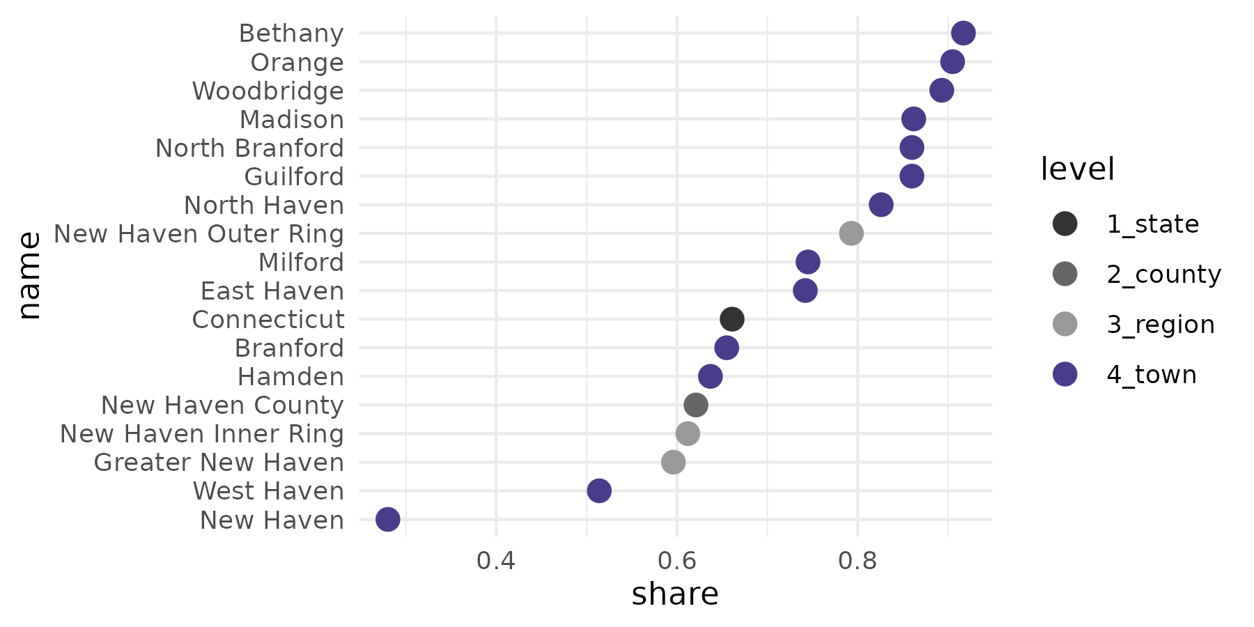
acs_quick_map() gives a quick map sketch of the rates.
This function uses the Jenks algorithm for making breaks with
jenks(). This algorithm is well suited for visually
displaying larger inequalities, but the number of breaks you give it
won’t necessarily be the number of breaks returned.This function lets us
see whether there’s a geographic distribution of this data with minimal
work.
tenure_map <- homeownership |>
  filter(level == "4_town") |>
  quick_map(
    value = share, level = "town", color = "black", linewidth = 0.4,
    title = "Homeownership, Greater New Haven", palette = "BuPu"
  )

tenure_map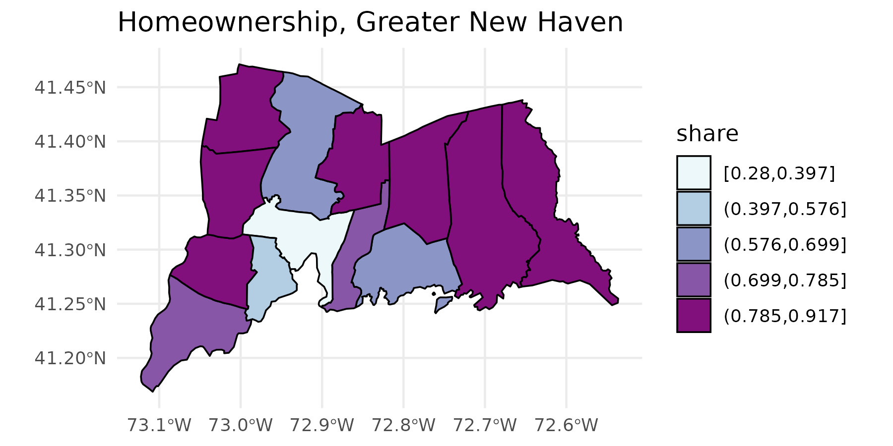
Since this returns a ggplot object with sf
data, we can add additional ggplot functions, such as
labeling, themes, or additional scales or geoms.
tenure_map +
  labs(subtitle = stringr::str_glue("By town, {yr}")) +
  geom_sf(data = . %>% filter(name == "New Haven"), fill = NA, color = "black", linewidth = 1.5)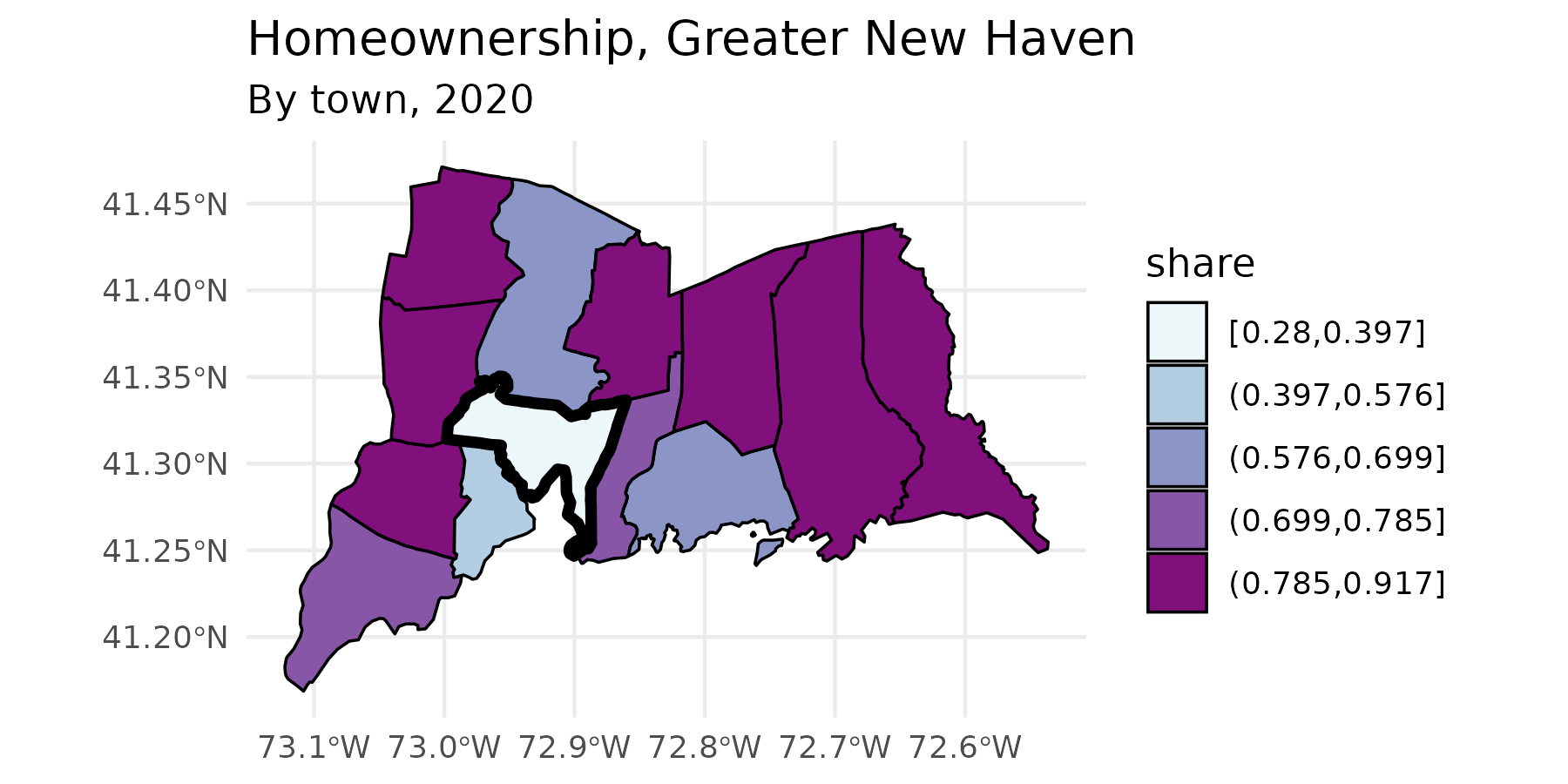
Batch output
Say as part of a pipeline, you need to do some calculations, write
different sections of a data frame to CSV files to pass along to a
colleague or refer to later, and then continue on to some more
calculations. batch_csv_dump() takes either a list of data
frames or a data frame plus a column to split by, and writes out a set
of CSV files, then lets you move along to the next step in your
pipeline.
For example, I need to pull a table of populations by age group for several regions of Connecticut. I don’t need to split populations by gender, so I’ll add up male and female populations for each age group. I don’t actually need to more detailed age groups now, but I need to stash them in files for later, so I’ll aggregate, write a bunch of files, and then aggregate into broader age groups that I need for my current work.
new_haven_regions <- regions[c(
  "Greater New Haven", "New Haven Inner Ring",
  "New Haven Outer Ring", "Lower Naugatuck Valley",
  "Greater Waterbury"
)]

age <- multi_geo_acs(
  table = "B01001", year = yr, towns = NULL,
  regions = new_haven_regions,
  counties = c("New Haven County", "Fairfield County")
) |>
  label_acs(year = yr) |>
  # shortcut around tidyr::separate
  separate_acs(into = c("sex", "age"), drop_total = TRUE) |>
  filter(!is.na(age)) |>
  mutate(age = forcats::as_factor(age)) |>
  group_by(name, level, age) |>
  summarise(estimate = sum(estimate)) |>
  ungroup()

age |>
  split(~name) |>
  batch_csv_dump(base_name = "pop_by_age", bind = TRUE, verbose = TRUE) |>
  group_by(level, name) |>
  camiller::add_grps(list(ages00_04 = 1, ages05_17 = 2:4, ages00_17 = 1:4),
    group = age, value = estimate
  ) |>
  arrange(level, name, age)
Employment trends
Quarterly Workforce Indicators
I’m also interested in learning about employment by industry over the
past several years. qwi_industry() fetches county-level
data by industry over time, either quarterly or annually. Here I’ll look
at annual averages of all industries for South Central COG and
Connecticut over the past 16 years. I’m filtering out the industry code
“00”, which is the counts for all industries.
scc_employment <- qwi_industry(2002:2018, counties = "170", annual = TRUE) |>
  mutate(location = "South Central COG")
#> ℹ Note that starting with the 2022 release, ACS data uses COGs instead of
#>   counties.
#> ℹ The API can only get 10 years of data at once; making multiple calls, but this might take a little longer.
#>
#> This message is displayed once per session.
ct_employment <- qwi_industry(2002:2018, annual = T) |>
  mutate(location = "Connecticut")
#> ℹ The API can only get 10 years of data at once; making multiple calls, but this might take a little longer.
employment <- bind_rows(scc_employment, ct_employment) |>
  filter(industry != "00") |>
  inner_join(naics_codes |> select(-ind_level), by = "industry")

employment
#> # A tibble: 680 × 8
#>     year state county industry     emp payroll location          label
#>    <dbl> <chr> <chr>  <chr>      <dbl>   <dbl> <chr>             <chr>
#>  1  2002 09    170    11         380        NA South Central COG Agriculture, F…
#>  2  2002 09    170    21          31.2      NA South Central COG Mining, Quarry…
#>  3  2002 09    170    22        1102.       NA South Central COG Utilities
#>  4  2002 09    170    23       11208.       NA South Central COG Construction
#>  5  2002 09    170    31-33    33478.       NA South Central COG Manufacturing
#>  6  2002 09    170    42       11318.       NA South Central COG Wholesale Trade
#>  7  2002 09    170    44-45    32920        NA South Central COG Retail Trade
#>  8  2002 09    170    48-49     5772.       NA South Central COG Transportation…
#>  9  2002 09    170    51       11897.       NA South Central COG Information
#> 10  2002 09    170    52       10708        NA South Central COG Finance and In…
#> # ℹ 670 more rows
Next, say I want to look at the industries that were largest in the
South Central COG in 2018, and see how those have changed both for the
COG and statewide over this time period. I’ll filter
employment, get the industries with the largest numbers of
employees, then filter employment for just those industries
and plot it.
top2018 <- employment |>
  filter(year == 2018, county == "170") |>
  top_n(8, emp) |>
  pull(industry)
top2018
#> [1] "31-33" "44-45" "54"    "56"    "61"    "62"    "72"    "81"
employment |>
  filter(industry %in% top2018) |>
  mutate(label = stringr::str_sub(label, 1, 25)) |>
  mutate(Emp_1k = emp / 1000) |>
  ggplot(aes(x = year, y = Emp_1k, color = label)) +
  geom_line() +
  labs(
    x = "Year", y = "Employees (thousands)", title = "Employment by industry",
    subtitle = "Connecticut and South Central COG, 2002-2018", color = "Industry"
  ) +
  theme_minimal() +
  facet_wrap(vars(location), scales = "free_y")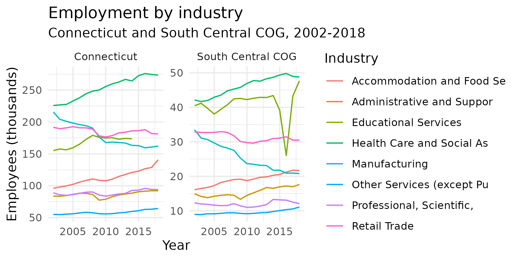
Update 11/2021: The QWI API was broken for a little while. It’s up again, but all the payroll data is missing. This code should still be valid if it ever gets returned.
If I’m interested in changes in wages over this period, I can use the
adj_inflation() function. This takes a data frame, the name
of the column containing dollar amounts, and a base year, then adds two
columns for the inflation adjustment factor and the adjusted value.
employment |>
  filter(industry %in% top2018) |>
  mutate(label = stringr::str_sub(label, 1, 25)) |>
  mutate(avg_wage = Payroll / Emp) |>
  adj_inflation(value = avg_wage, base_year = 2018, year = year) |>
  mutate(adj_wage_1k = round(adj_avg_wage / 1000)) |>
  ggplot(aes(x = year, y = adj_wage_1k, color = label)) +
  geom_line() +
  scale_y_continuous(labels = scales::dollar) +
  labs(
    x = "Year", y = "Average annual wages (thousands)",
    title = "Average annual wages by industry (adjusted to 2018 dollars)",
    subtitle = "Connecticut and New Haven County, 2002-2018", color = "Industry"
  ) +
  theme_minimal() +
  facet_wrap(vars(location), scales = "free_y")
Now we have a visual that shows that in a few industries, wages have climbed over the past several years, but in many industries, wages haven’t increased except by inflation.
Local Area Unemployment Statistics
To look at unemployment rates over time, I can use
laus_trend(). The LAUS covers smaller geographies than the
QWI, so laus_trend() is set up to find data by a
combination of state, counties, or towns. The LAUS API returns monthly
data on labor force counts, employment counts, unemployed counts, and
unemployment rate; laus_trend() lets you specify which of
these measures to fetch.
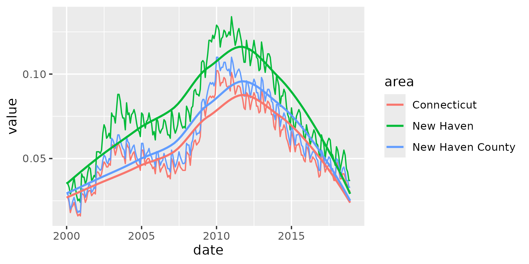
unemployment <- laus_trend(c("New Haven", "New Haven County", "Connecticut"),
  startyear = 2000, endyear = 2018, measures = "unemployment rate"
) |>
  mutate(unemployment_rate = unemployment_rate / 100) |>
  select(area, date, value = unemployment_rate)
#>
#> ── Local Area Unemployment Statistics ──────────────────────────────────────────
#> • Unemployment Rate
#> • Not Seasonally Adjusted
unemployment
#> # A tibble: 684 × 3
#>    area             date       value
#>    <chr>            <date>     <dbl>
#>  1 Connecticut      2000-01-01 0.027
#>  2 New Haven County 2000-01-01 0.029
#>  3 New Haven        2000-01-01 0.036
#>  4 Connecticut      2000-02-01 0.027
#>  5 New Haven County 2000-02-01 0.029
#>  6 New Haven        2000-02-01 0.035
#>  7 Connecticut      2000-03-01 0.024
#>  8 New Haven County 2000-03-01 0.025
#>  9 New Haven        2000-03-01 0.033
#> 10 Connecticut      2000-04-01 0.018
#> # ℹ 674 more rows
unemp_plot <- ggplot(unemployment, aes(x = date, y = value, group = area, color = area)) +
  geom_line() +
  geom_smooth(se = FALSE, method = "loess", linewidth = 0.8)
unemp_plot
#> `geom_smooth()` using formula = 'y ~ x'