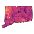
This is a quick way to create a choropleth sketch of town-, neighborhood-, or tract-level data. Uses a corresponding sf object; as of June 2018, this sf object must be one that ships with this package, or otherwise be globally available.
Usage
quick_map(
  data,
  name = name,
  value = value,
  level = c("town", "neighborhood", "tract"),
  city = NULL,
  n = 5,
  palette = "GnBu",
  title = NULL,
  ...
)
Arguments
- data
A data frame containing data by geography.
- name
Bare column name of location names to join; defaults
name.- value
Bare column name of numeric values to map; defaults
value.- level
String giving the desired geographic level; must be one of
"town","neighborhood", or"tract". Defaults"town".- city
If geographic level is neighborhood, string of the corresponding city name to match to a spatial object.
- n
Number of breaks into which to bin values; defaults (approximately) 5.
- palette
String of a ColorBrewer palette; see
RColorBrewer::RColorBrewer()for possible values. Defaults"GnBu".- title
String giving the title, if desired, for the plot.
- ...
Arguments passed on to
ggplot2::geom_sfxlim,ylimLimits for the x and y axes. These limits are specified in the units of the default CRS. By default, this means projected coordinates (
default_crs = NULL). How limit specifications translate into the exact region shown on the plot can be confusing when non-linear or rotated coordinate systems are used as the default crs. First, different methods can be preferable under different conditions. See parameterlims_methodfor details. Second, specifying limits along only one direction can affect the automatically generated limits along the other direction. Therefore, it is best to always specify limits for both x and y. Third, specifying limits via position scales orxlim()/ylim()is strongly discouraged, as it can result in data points being dropped from the plot even though they would be visible in the final plot region.expandIf
TRUE, the default, adds a small expansion factor to the limits to ensure that data and axes don't overlap. IfFALSE, limits are taken exactly from the data orxlim/ylim. Giving a logical vector will separately control the expansion for the four directions (top, left, bottom and right). Theexpandargument will be recycled to length 4 if necessary. Alternatively, can be a named logical vector to control a single direction, e.g.expand = c(bottom = FALSE).crsThe coordinate reference system (CRS) into which all data should be projected before plotting. If not specified, will use the CRS defined in the first sf layer of the plot.
default_crsThe default CRS to be used for non-sf layers (which don't carry any CRS information) and scale limits. The default value of
NULLmeans that the setting forcrsis used. This implies that all non-sf layers and scale limits are assumed to be specified in projected coordinates. A useful alternative setting isdefault_crs = sf::st_crs(4326), which means x and y positions are interpreted as longitude and latitude, respectively, in the World Geodetic System 1984 (WGS84).datumCRS that provides datum to use when generating graticules.
label_graticuleCharacter vector indicating which graticule lines should be labeled where. Meridians run north-south, and the letters
"N"and"S"indicate that they should be labeled on their north or south end points, respectively. Parallels run east-west, and the letters"E"and"W"indicate that they should be labeled on their east or west end points, respectively. Thus,label_graticule = "SW"would label meridians at their south end and parallels at their west end, whereaslabel_graticule = "EW"would label parallels at both ends and meridians not at all. Because meridians and parallels can in general intersect with any side of the plot panel, for any choice oflabel_graticulelabels are not guaranteed to reside on only one particular side of the plot panel. Also,label_graticulecan cause labeling artifacts, in particular if a graticule line coincides with the edge of the plot panel. In such circumstances,label_axeswill generally yield better results and should be used instead.This parameter can be used alone or in combination with
label_axes.label_axesCharacter vector or named list of character values specifying which graticule lines (meridians or parallels) should be labeled on which side of the plot. Meridians are indicated by
"E"(for East) and parallels by"N"(for North). Default is"--EN", which specifies (clockwise from the top) no labels on the top, none on the right, meridians on the bottom, and parallels on the left. Alternatively, this setting could have been specified withlist(bottom = "E", left = "N").This parameter can be used alone or in combination with
label_graticule.lims_methodMethod specifying how scale limits are converted into limits on the plot region. Has no effect when
default_crs = NULL. For a very non-linear CRS (e.g., a perspective centered around the North pole), the available methods yield widely differing results, and you may want to try various options. Methods currently implemented include"cross"(the default),"box","orthogonal", and"geometry_bbox". For method"cross", limits along one direction (e.g., longitude) are applied at the midpoint of the other direction (e.g., latitude). This method avoids excessively large limits for rotated coordinate systems but means that sometimes limits need to be expanded a little further if extreme data points are to be included in the final plot region. By contrast, for method"box", a box is generated out of the limits along both directions, and then limits in projected coordinates are chosen such that the entire box is visible. This method can yield plot regions that are too large. Finally, method"orthogonal"applies limits separately along each axis, and method"geometry_bbox"ignores all limit information except the bounding boxes of any objects in thegeometryaesthetic.ndiscrNumber of segments to use for discretising graticule lines; try increasing this number when graticules look incorrect.
defaultIs this the default coordinate system? If
FALSE(the default), then replacing this coordinate system with another one creates a message alerting the user that the coordinate system is being replaced. IfTRUE, that warning is suppressed.clipShould drawing be clipped to the extent of the plot panel? A setting of
"on"(the default) means yes, and a setting of"off"means no. In most cases, the default of"on"should not be changed, as settingclip = "off"can cause unexpected results. It allows drawing of data points anywhere on the plot, including in the plot margins. If limits are set viaxlimandylimand some data points fall outside those limits, then those data points may show up in places such as the axes, the legend, the plot title, or the plot margins.reverseA string giving which directions to reverse.
"none"(default) keeps directions as is."x"and"y"can be used to reverse their respective directions."xy"can be used to reverse both directions.mappingSet of aesthetic mappings created by
aes(). If specified andinherit.aes = TRUE(the default), it is combined with the default mapping at the top level of the plot. You must supplymappingif there is no plot mapping.statThe statistical transformation to use on the data for this layer. When using a
geom_*()function to construct a layer, thestatargument can be used to override the default coupling between geoms and stats. Thestatargument accepts the following:A
Statggproto subclass, for exampleStatCount.A string naming the stat. To give the stat as a string, strip the function name of the
stat_prefix. For example, to usestat_count(), give the stat as"count".For more information and other ways to specify the stat, see the layer stat documentation.
positionA position adjustment to use on the data for this layer. This can be used in various ways, including to prevent overplotting and improving the display. The
positionargument accepts the following:The result of calling a position function, such as
position_jitter(). This method allows for passing extra arguments to the position.A string naming the position adjustment. To give the position as a string, strip the function name of the
position_prefix. For example, to useposition_jitter(), give the position as"jitter".For more information and other ways to specify the position, see the layer position documentation.
na.rmIf
FALSE, the default, missing values are removed with a warning. IfTRUE, missing values are silently removed.show.legendlogical. Should this layer be included in the legends?
NA, the default, includes if any aesthetics are mapped.FALSEnever includes, andTRUEalways includes.You can also set this to one of "polygon", "line", and "point" to override the default legend.
inherit.aesIf
FALSE, overrides the default aesthetics, rather than combining with them. This is most useful for helper functions that define both data and aesthetics and shouldn't inherit behaviour from the default plot specification, e.g.annotation_borders().parseIf
TRUE, the labels will be parsed into expressions and displayed as described in?plotmath.label.paddingAmount of padding around label. Defaults to 0.25 lines.
label.rRadius of rounded corners. Defaults to 0.15 lines.
label.size![[Deprecated]](figures/lifecycle-deprecated.svg) Replaced by the
Replaced by the
linewidthaesthetic. Size of label border, in mm.border.colour,border.colorColour of label border. When
NULL(default), thecolouraesthetic determines the colour of the label border.border.coloris an alias forborder.colour.text.colour,text.colorColour of the text. When
NULL(default), thecolouraesthetic determines the colour of the text.text.coloris an alias fortext.colour.fun.geometryA function that takes a
sfcobject and returns asfc_POINTwith the same length as the input. IfNULL,function(x) sf::st_point_on_surface(sf::st_zm(x))will be used. Note that the function may warn about the incorrectness of the result if the data is not projected, but you can ignore this except when you really care about the exact locations.check_overlapIf
TRUE, text that overlaps previous text in the same layer will not be plotted.check_overlaphappens at draw time and in the order of the data. Therefore data should be arranged by the label column before callinggeom_text(). Note that this argument is not supported bygeom_label().geomThe geometric object to use to display the data for this layer. When using a
stat_*()function to construct a layer, thegeomargument can be used to override the default coupling between stats and geoms. Thegeomargument accepts the following:A
Geomggproto subclass, for exampleGeomPoint.A string naming the geom. To give the geom as a string, strip the function name of the
geom_prefix. For example, to usegeom_point(), give the geom as"point".For more information and other ways to specify the geom, see the layer geom documentation.
Examples
if (FALSE) { # \dontrun{
tidycensus::get_acs(
    geography = "county subdivision", year = 2023,
    variables = c(median_age = "B01002_001"), state = "09", county = "170"
) |>
    town_names(NAME) |>
    dplyr::filter(NAME %in% regions$`Greater New Haven`) |>
    quick_map(name = NAME, value = estimate, title = "Median age by town, 2023", n = 6)
} # }