PUMA update

library(dplyr)
library(sf)
library(ggplot2)
library(purrr)

sf_use_s2(FALSE)

theme_set(theme_minimal())

Most geographies that are subdivisions of county-equivalents only changed their FIPS codes when the state changed from counties to COGs. PUMAs changed their actual boundaries. For the most part these are set within COGs, but Northeastern COG has too small a population to be its own PUMA (minimum for a PUMA is 100k), so its PUMA also includes Stafford.

town_puma <- cwi::xwalk |>
  distinct(town, puma_fips, puma_fips_cog, cog) |>
  rename(puma_county = puma_fips, puma_cog = puma_fips_cog) |>
  mutate(across(c(puma_county, puma_cog), list(group = \(x) substr(x, 3, 5)))) |>
  left_join(cwi::town_sf, by = c("town" = "name")) |>
  st_as_sf() |>
  select(-GEOID)

st_write(town_puma, here::here("output_data/town_to_puma.gpkg"), delete_layer = TRUE)

Deleting layer `town_to_puma' using driver `GPKG'
Writing layer `town_to_puma' to data source 
  `/home/camille/code/cogs/output_data/town_to_puma.gpkg' using driver `GPKG'
Writing 169 features with 6 fields and geometry type Multi Polygon.

Wrote out GPKG file to upload to Carto.

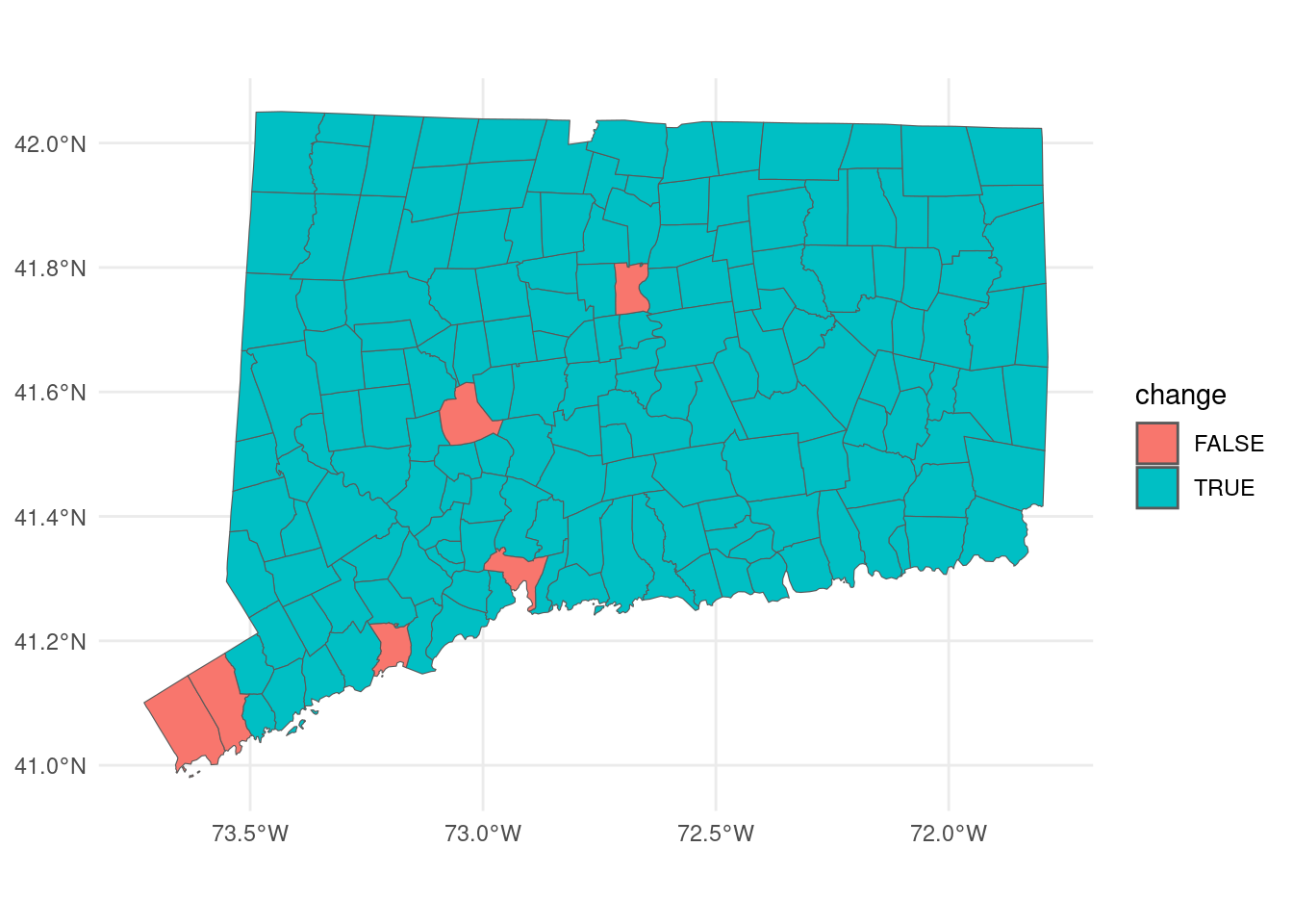
Other than the 4 PUMAs that are standalone cities, plus the one that is just Stamford and Greenwich, every town’s PUMA underwent some change.

town_puma_list <- list(
  county = town_puma |> select(town, puma = puma_county),
  cog = town_puma |> select(town, puma = puma_cog)
) |>
  map(st_drop_geometry) |>
  map(group_by, puma) |>
  map(summarise, towns = toString(sort(town)))

full_join(town_puma_list$county, town_puma_list$cog, by = "towns", suffix = c("_county", "_cog")) |>
  filter(is.na(puma_county) | is.na(puma_cog)) |>
  tidyr::separate_rows(towns, sep = ", ") |>
  distinct(towns) |>
  mutate(change = TRUE) |>
  right_join(cwi::town_sf, by = c("towns" = "name")) |>
  tidyr::replace_na(list(change = FALSE)) |>
  st_as_sf() |>
  ggplot() +
  geom_sf(aes(fill = change))