Easily add a logo to a ggplot

This function wraps around a few functions from patchwork and magick to add a logo (or other annotation) to the bottom of a ggplot plot, an otherwise tedious and easy to forget process. It's meant to be flexible in the types of objects it can place; as a result, it's less flexible in their placement and customization. For more specific needs, the source of this function should be easy to build upon. Previously it used cowplot, but that package is a bit too buggy.

Usage

add_logo(
  plot,
  image = NULL,
  position = c("right", "left"),
  height = 0.05,
  width = NULL,
  place_inside = TRUE
)

Arguments

plot: A ggplot object onto which the logo will be placed.
image: Either a string giving the path or URL to an image file to be read by magick::image_read; the results of reading a file or manipulating an image already with magick::image_read or other magick functions; a ggplot object / grob; or NULL, the default. If NULL, the image will come from the file at system.file("extdata/logo.svg", package = "stylehaven"). As built, this is a logo for DataHaven, but that file can be replaced for repackaging this library for other organizations or projects.
position: String, either "left" or "right", giving the side on which the logo should be aligned. Default: "right"
height: Numeric: the height of the logo, as a percentage of the height of the image given in plot. Adjust as necessary based on the dimensions of the logo. Default: 0.05
width: Numeric: the width of the logo, as a percentage of the image given in plot. If NULL, the default, the width will be calculated based on the aspect ratio of the image. Must be given explicitly for ggplot objects, as they don't inherently have their own dimensions.
place_inside: Logical: if TRUE (default), logo will be drawn within the plotting area; otherwise, an additional grob is built below the plot, meaning the logo could later be cropped away, which may be undesirable.

Value

A ggplot object.

Examples

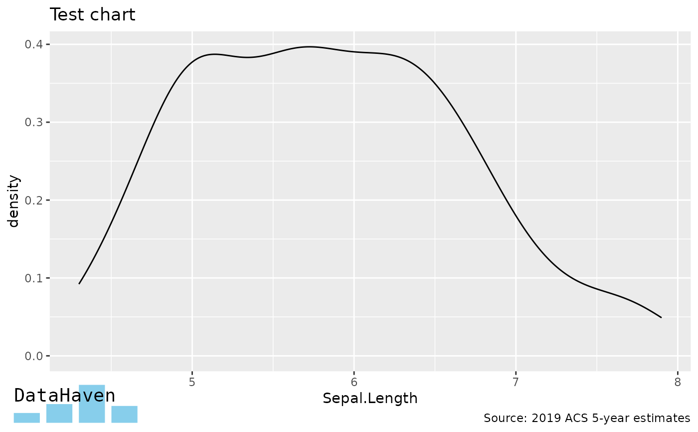
library(ggplot2)
p <- ggplot(iris, ggplot2::aes(x = Sepal.Length)) +
    geom_density() +
    labs(title = "Test chart", caption = "Source: 2019 ACS 5-year estimates") +
    theme(plot.caption = element_text(hjust = 0))

add_logo(p)
#> Warning: ImageMagick was built without librsvg which causes poor qualty of SVG rendering.
#> For better results use image_read_svg() which uses the rsvg package.

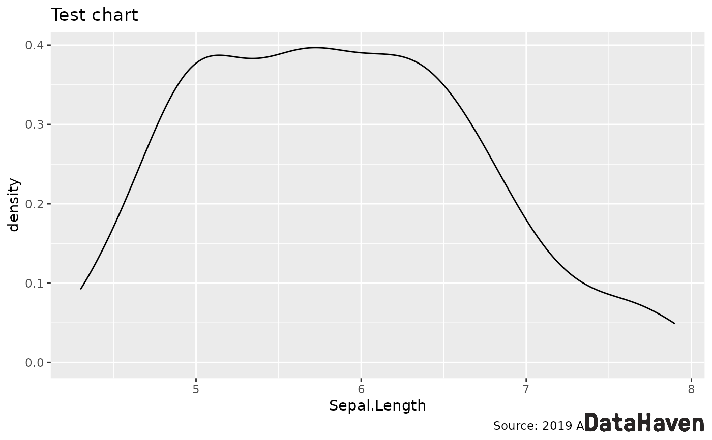# this one is too tall--place it outside so it doesn't block axis
add_logo(p,
    magick::image_read(system.file("extdata/25th_logo.png", package = "stylehaven")),
    height = 0.1, place_inside = FALSE
)


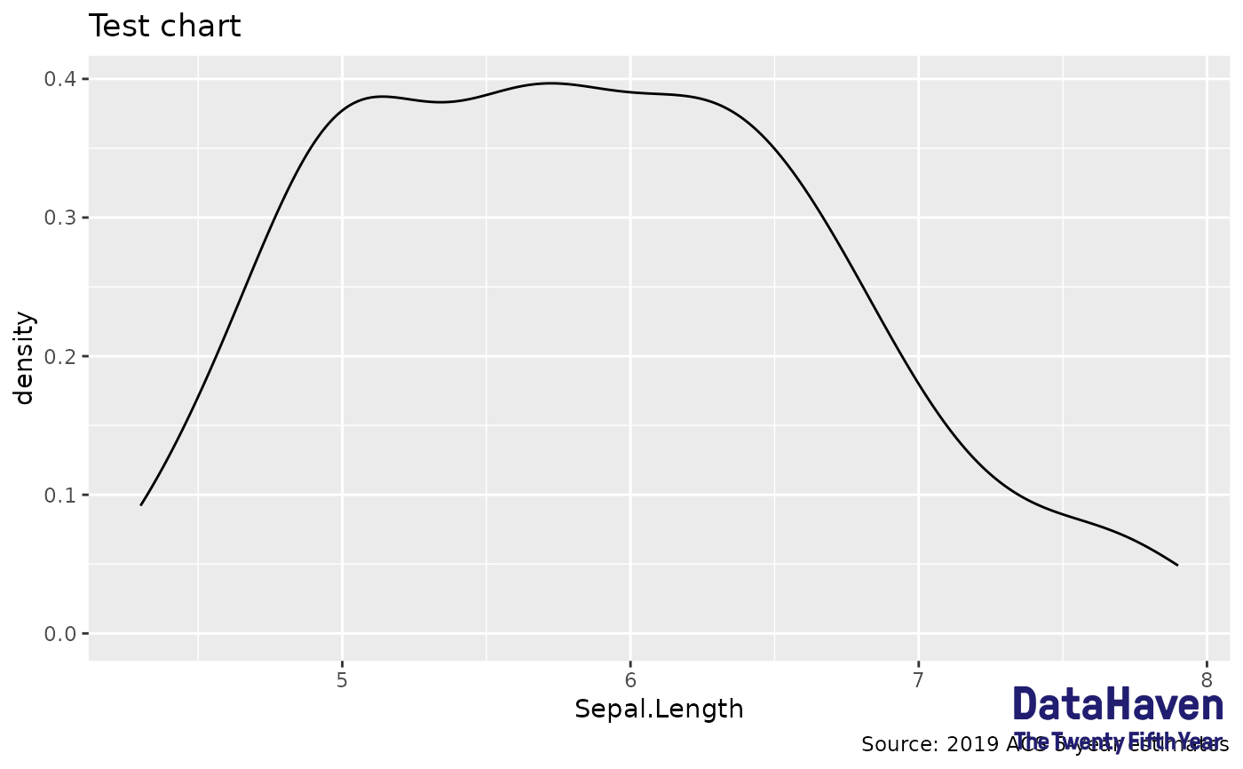# This example logo is not all that attractive, but shows how you might
# attach a ggplot grob as a dynamically-created logo
dummy_data <- data.frame(
    town = letters[1:4],
    pop = c(21000, 40000, 81000, 36000)
)

gg_logo <- ggplot(dummy_data, aes(x = town, y = pop)) +
    geom_col(width = 0.8, fill = "skyblue") +
    annotate(
        geom = "text", label = "DataHaven", x = 0.6, y = 6e4, hjust = 0,
        family = "mono", size = 5
    ) +
    theme_void()

add_logo(p, gg_logo, width = 0.2, height = 0.1)

Usage

Arguments

Value

See also

Examples