• acs.R package provides easier interface for working with Census API
• Focused on ACS, but also can access SF1, SF3 decennial tables
• Comes with its own weird objects—something to get used to
• Developed by Ezra Habel Glenn at MIT
• Very good user guide! http://bit.ly/acshandbook

See the repo for this presentation at https://github.com/CT-Data-Haven/acs_presentation

Goal: make a profile of several indicators for local geographies in R

Input: the acs.R package & API key from the Census

Output: CSV file ready to share with clients, public, etc

• Make combined geographies
• Pull several ACS tables using the acs package
• Aggregate variables as needed
• Calculate stuff—rates, etc
• Get everything into a single dataframe & write to csv

This will be pretty technical—sorry in advance!

Some resources for practicing R:

• DataCamp: http://datacamp.com Costs money but is totally worth it for interactive courses
• Tutorials from RStudio: http://rstudio.com/online-learning
• R for Data Science free online book: http://r4ds.had.co.nz/
• swirl, package for R tutorials inside RStudio: http://swirlstats.com/

• Making heavy use of the tidyverse packages
• purrr lets us use map functions to work with lists
• Learn more:
  • http://tidyverse.org/
  • http://r4ds.had.co.nz/

library(acs)
library(tidyverse)
library(stringr)

There's a very new (May 2017) package called tidycensus that I haven't worked with yet, but recommend people also check out: https://github.com/walkerke/tidycensus

acs package comes with many helper functions:

• geo.lookup to help with looking up geography details—useful for getting FIPS codes, or when you forgot what county a town is in
• acs.lookup for variables and table numbers, but the output is annoying to work with
• currency.convert for inflation adjustments
• Plus dataframes of FIPS codes

Getting ACS table numbers

In addition to acs.lookup (if you can sort through the output okay), you can get table numbers from ACS technical docs (look up "table shells").

Or, the easiest way to get table numbers might just be FactFinder :(

• acs package has several of its own object types, including geo.set for geographies
• Make geo.set objects based on FIPS codes and/or names
• Can combine multiple geographies in a few ways:
  • as a list of geographies (combine = FALSE)
  • a merged geography (combine = TRUE)

See documentation on geo.make to see lots of different ways to make geographies, given FIPS codes and names. Ones I use commonly involve:

Single state

ct <- geo.make(state = 09)

Single town

nhv <- geo.make(state = 09, county = 09, county.subdivision = "New Haven")

Multiple towns merged into single geography with combine = T

inner_ring <- geo.make(state = 09, county = 09, 
                       county.subdivision = c("Hamden", "West Haven", "East Haven"), 
                       combine = T, combine.term = "Inner Ring towns")

Neighborhoods get a little more tricky

Single Census tract

dixwell <- geo.make(state = 09, county = 09, tract = 141600)

Single tract, multiple block groups merged

west_rock <- geo.make(state = 09, county = 09, 
                      tract = 141300, block.group = c(1, 4), 
                      combine = T, combine.term = "West Rock")

Mashup of block groups from multiple tracts (using wildcard "*")

beaver_hills <- geo.make(state = 09, county = 09, 
                         tract = c(141400, 141300), block.group = c("*", 2), 
                         combine = T, combine.term = "Beaver Hills")

Then make geo.set using c

geos <- c(ct, nhv, inner_ring, beaver_hills, dixwell, west_rock)

Total population: table number B01003

acs.fetch gets an ACS table for a geography & year—yields an acs object

pop <- acs.fetch(geography = geos, endyear = 2015, 
                 table.number = "B01003", col.names = "pretty")
pop

## ACS DATA: 
##  2011 -- 2015 ;
##   Estimates w/90% confidence intervals;
##   for different intervals, see confint()
##                                                  Total Population: Total    
## Connecticut                                      3593222 +/- 0              
## New Haven town, New Haven County, Connecticut    130612 +/- 50              
## Inner Ring towns                                 145816 +/- 96.4676111448812
## Beaver Hills                                     5521 +/- 805.957194893128  
## Census Tract 1416, New Haven County, Connecticut 4898 +/- 503               
## West Rock                                        4132 +/- 463.159799637231

My favorite method: using purrr functions, map over a named list of table numbers—yields a named list of acs objects. Super convenient when you're working with 20+ tables.

table_nums <- list( 
  total_pop = "B01003", 
  tenure = "B25003",
  poverty = "C17002"
)

fetch <- table_nums %>% 
  map(~acs.fetch(geography = geos, endyear = 2015, 
                 table.number = ., col.names = "pretty"))

acs.R has several functions for analysis, and allows many standard functions to work on acs objects—check the docs for acs-class.

Margins of error are handled for you! Add, divide, etc. columns in your tables without worrying about how to deal with MOEs.

(I got tired of repeating some of these operations, and wrote an entire package to streamline this: https://github.com/CT-Data-Haven/acsprofiles)

I'll have several acs objects after analysis—total_pop, tenure, poverty—then cbind them all together into a single acs object.

Total population

Total population is ready to go, but it helps to shorten the name (also helps with a rounding trick later)

total_pop <- fetch$total_pop[, 1]
acs.colnames(total_pop) <- "num_total_pop"

Homeownership rate

Step by step:

• Get denominator: total households (column 1)
• Get number of owner-occupied households (column 2)
• Divide to get rate

Divide using divide.acs from acs.R

households <- fetch$tenure[, 1]
owned <- fetch$tenure[, 2]
owned_rate <- divide.acs(owned, households)

tenure <- list(households, owned, owned_rate) %>% reduce(cbind)

# names come out ugly after division
acs.colnames(tenure) <- c("num_households", "num_owned_hh", "percent_owned_hh")

Poverty & low-income rates

Step by step:

• Get denominator: total population for which poverty status is determined (column 1)
• Get population in poverty, i.e. below 1.0 x FPL (columns 2 + 3)
• Get low-income population, i.e. below 2.0 x FPL (columns 2 through 7)
• Divide to get rates

Add columns as necessary using apply, divide using divide.acs from acs.R. Really not as ugly as this looks!

deter <- fetch$poverty[, 1]
poverty <- apply(X = fetch$poverty[, 2:3], FUN = sum, MARGIN = 2, agg.term = "poverty")
pov_rate <- divide.acs(poverty, deter)

low_income <- apply(X = fetch$poverty[, 2:7], FUN = sum, MARGIN = 2, agg.term = "low inc")
low_inc_rate <- divide.acs(low_income, deter)

poverty <- list(deter, poverty, pov_rate, low_income, low_inc_rate) %>%
  reduce(cbind)

# names come out ugly after division
acs.colnames(poverty) <- c("num_poverty_determined", "num_in_poverty", 
                      "percent_in_poverty", "num_low_income", "percent_low_income")

acs objects have several slots, including @geography, @estimate, @standard.error

A simple dataframe here will contain the name of the geography, then columns for all estimates. Using @standard.error, you can include margins of error calculations.

all_tables <- list(total_pop, tenure, poverty) %>% reduce(cbind)

# multiplying standard.error by qnorm(0.95) to get 90% MOE as used in ACS tables online
profile <- data.frame(name = all_tables@geography$NAME,
                      all_tables@estimate,
                      all_tables@standard.error * qnorm(0.95)) %>%
  tbl_df() %>%
  mutate(name = str_replace(name, " town,.+", "")) %>%
  mutate_at(vars(starts_with("percent")), funs(round(., digits = 3))) %>%
  mutate_at(vars(starts_with("num")), funs(round(.))) %>%
  setNames(str_replace(names(.), ".1", "_moe"))

# manually changing name for Dixwell---could use workaround if there were more to redo
profile$name[str_detect(profile$name, "Census Tract 1416")] <- "Dixwell"

rmarkdown::paged_table(profile)

write_csv(profile, "mini ACS profile.csv")

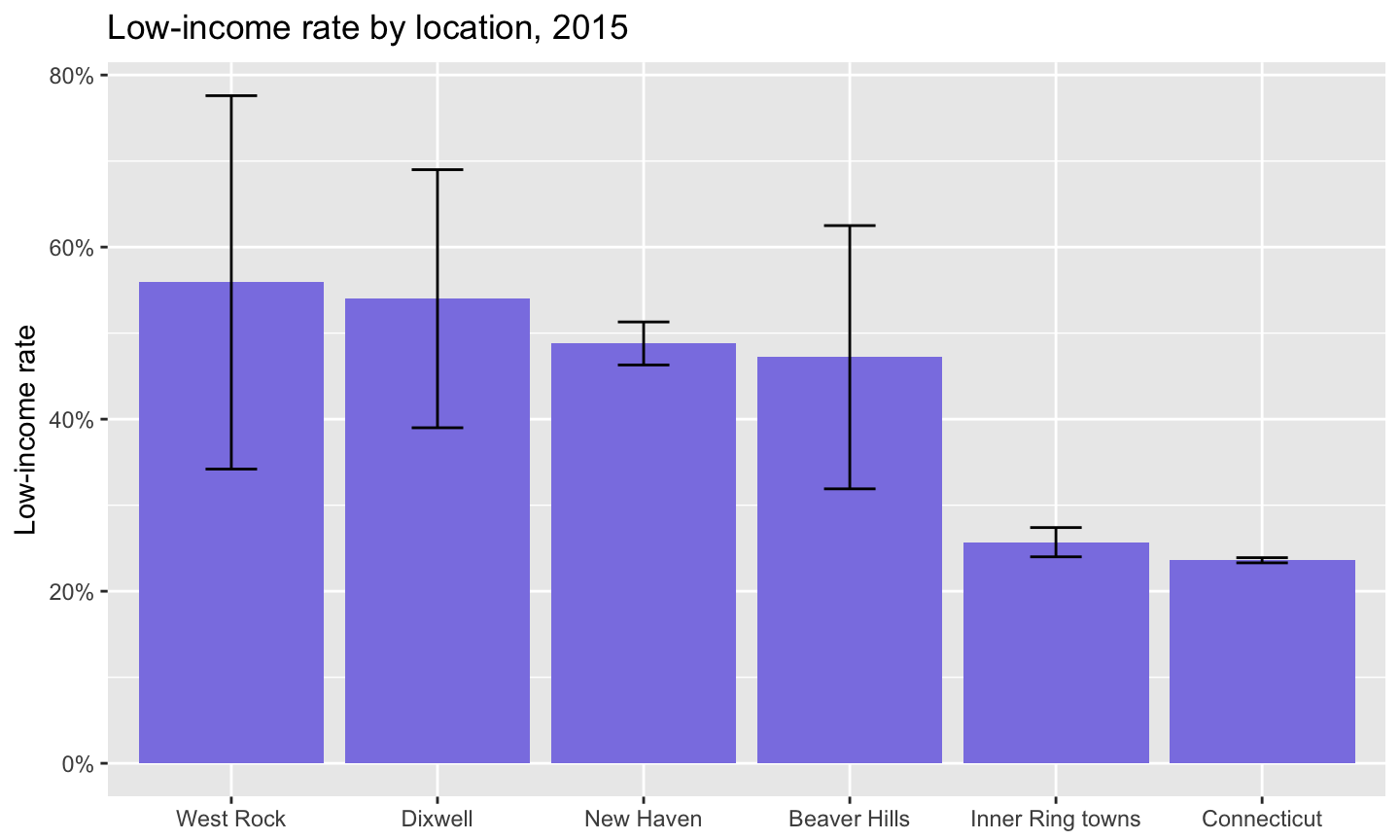
Having a great workflow doesn't get us over the problem of large margins of error with small geographies. MOEs for low-income rates aren't bad for towns & bigger, but ugly for neighborhoods

https://github.com/CT-Data-Haven

camille@ctdatahaven.org